
Why Does My Online Turbidity Sensor Drift? A Technical FAQ
An online turbidity sensor rarely fails by stopping. It fails by staying plausible. The reading keeps updating, keeps logging, keeps feeding the SCADA screen or the public dashboard, while the number it reports slowly separates from the water it is supposed to describe. For a municipal plant reporting effluent quality, a surface-water station feeding a compliance record, or an aquaculture site driving feed and aeration decisions, a drifted signal is more dangerous than a dead one.
This FAQ addresses the questions buyers and plant engineers actually raise during research and evaluation: why optical turbidity measurements drift, how to tell one failure mode from another, what self-cleaning hardware genuinely does and does not do, and how to choose between scattered-light and transmittance-based approaches when the application, not the datasheet, is the deciding factor.
What Turbidity Drift Is, and What It Is Not
An optical turbidity measurement rests on a single physical relationship: suspended particles scatter light into a detector at a defined angle, and the intensity of that scattered light is mapped onto a turbidity value. As long as the optical path and the sample are unchanged, that mapping should remain stable. Drift is a shift in the mapping itself — a rising zero point, a decaying slope, or both — measured against a reference the instrument has not changed.
Noise is a different phenomenon. Spikes, step changes and unstable traces come from the sample or the installation: a bubble passing the window, a slug of coarse solids, a pump cycling on. Both drift and noise produce a number that is wrong, but they have different causes and completely different remedies. Confusing them is the most common reason a maintenance team replaces a sensor that was never faulty.
The practical distinction: a baseline that walks upward over weeks is almost always a window-fouling problem. A reading that jumps in synchrony with a pump is almost always a bubble or flow problem. A clean zero that holds while the slope keeps falling is usually an optical-source or optical-path problem.
The Four Root Causes of Optical Turbidity Drift
1. Optical window fouling
Biofilm, calcium carbonate scale, iron and manganese oxide deposits, fats and organic films all accumulate on the optical window. Because fouling attenuates both the emitted beam and the returning scattered light, the usual effect is a loss of sensitivity combined with an unstable or elevated zero. Fouling is fastest in warm surface water during biological growth seasons, in municipal wastewater with high organic load, in aquaculture systems with heavy feed input, and anywhere the flow is slow enough for a stagnant boundary layer to form around the probe.
Window fouling is the single most common cause of slow upward drift in scattered-light turbidity measurement, and it is also the cheapest to correct — provided the installation allows the probe to be reached.
2. Bubble and flow interference
An air bubble scatters far more light than the suspended solids a turbidity sensor is designed to measure. Probes installed near pump discharges, at cascade points, in aerated basins, or in lines where dissolved gas can come out of solution will record spikes that look like drift over a long logging interval. The tell-tale signature is synchronisation: the reading moves when the pump moves, and settles when the flow settles.
This is an installation problem, not a sensor problem. Relocating the probe away from the discharge, maintaining back-pressure in a pressurised line, or introducing a small de-gassing section upstream of the measurement point usually resolves it without any change to the instrument.
3. Light-source ageing and optical-path loss
Light-emitting sources and photodetectors change output and response slowly over their service life. Window scratches, clouded encapsulants and degraded seals produce the same effect from the other direction. The characteristic signature is a clean zero that returns after wiping, combined with a slope that keeps needing correction in the same direction at every two-point calibration. This is the failure mode that most often gets mislabelled as an electronics fault when it is in fact an optical one.
4. Temperature and matrix effects
Temperature changes the refractive index of water and the behaviour of the electronics. KACISE's KWS-960C online turbidity sensor addresses the thermal part directly, with a built-in Pt1000 element providing automatic temperature compensation.
The matrix part is harder. Colour, particle size distribution and the organic-to-inorganic ratio of the suspended solids all shift the relationship between scattered light and reported NTU. Two samples can read identically on a laboratory reference and differently on an optical sensor if their particle size distributions differ. This is not instrument error; it is the boundary of the measurement principle, and it is the reason field calibration against the actual water body matters more than a factory default.
A Practical Field Diagnostic Table
The table below converts the four root causes into an observable-behaviour lookup. It is a starting point for diagnosis, not a substitute for a site inspection.
| Observed behaviour | Most probable cause | First corrective action |
|---|---|---|
| Zero climbs slowly; slope remains stable | Window fouling | Remove the probe, clean the optical window, re-check zero |
| Spikes synchronised with pump or aeration cycles | Bubble interference | Relocate or re-orient the probe; check line back-pressure |
| Clean zero returns, but slope keeps decaying | Light-source ageing or optical-path loss | Run a two-point calibration; inspect the window for scratches |
| Reading shifts with colour or solids type, not with time | Matrix effect | Recalibrate against the actual sample; evaluate colour compensation |
| Reading shifts after a temperature step | Thermal equilibrium or compensation | Verify the temperature reading against a reference thermometer |
| Reading falls abruptly after a maintenance visit | Deferred cleaning, not a fault | Shorten the cleaning interval; review access and installation |
What Self-Cleaning Hardware Actually Changes: 'Maintenance-Free' versus 'Reduced-Maintenance'
Product literature frequently presents a cleaning brush as a maintenance-free design. That framing is engineeringly inaccurate, and buyers should treat it as a warning sign rather than a benefit.
A rotating brush or wiper reduces the frequency of manual cleaning. It does not eliminate cleaning. Brush bristles wear, shafts and seals age, and in heavy grease or scaling service the brush head itself can crust over. What self-cleaning buys a project is a longer interval between interventions and a more stable signal between them — a genuine operational benefit, but a different claim from zero maintenance.
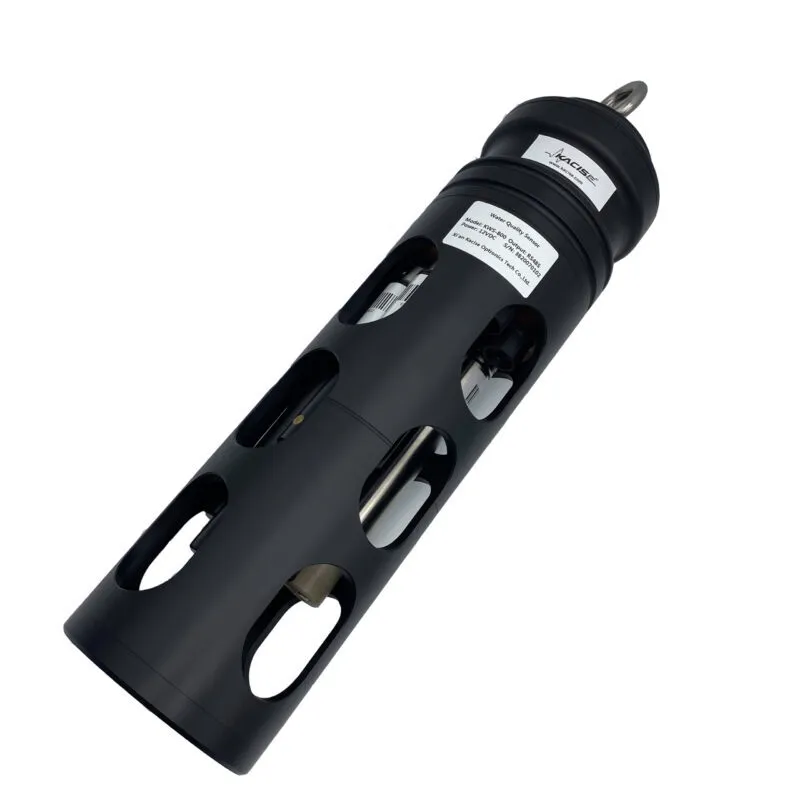
Within KACISE's water quality portfolio, the reduced-maintenance design appears in several forms. The KWS-910 online TSS sensor includes an automatic cleaning brush together with colour compensation and anti-ambient-light interference. The KWS-190 digital COD sensor is described as self-cleaning with automatic turbidity compensation. The KWS-110 and KWS-111 online COD sensors use a self-cleaning brush. The KWS-1003 variant of the KWS-1000 oil-in-water sensor includes an automatic cleaning brush. The KWS-800 online multi-parameter monitoring system incorporates an automatic cleaning device as part of its all-in-one design.
At the other end of the range, the KWS-960C online turbidity sensor is a direct-immersion optical design without an integrated brush. That is a deliberate product boundary, not an oversight: it suits installations where the probe can be reached for periodic cleaning, and it is the configuration in which the operator retains the most direct control over window condition.
Drift-Relevant Design in KACISE's Online Sensor Range
KACISE — Xi'an Kacise Optronics Tech Co., Ltd, a water quality sensor manufacturer headquartered in Xi'an, Shaanxi, China — operates a 40,000 m² production facility with an annual capacity of 120,000 units and exports to the EU and USA, with exports representing roughly 70% of output. Its water quality range covers turbidity, suspended solids, COD, pH, conductivity, dissolved oxygen, chlorophyll, oil-in-water and multi-parameter monitoring.
Online Turbidity Sensor KWS-960C
The KWS-960C measures turbidity and temperature using a 90° scattered-light principle with a fibre-optic structure, a built-in Pt1000 element for automatic temperature compensation, and RS485 (Modbus/RTU) output. Selectable ranges cover 0–20.00, 0–200.0 and 0–1000.0 NTU, with an operating temperature of 0–50 °C. The wetted body is 316L stainless steel with a 3/4 NPT connection and IP68 protection to 20 m water depth. Working pressure is below 0.2 MPa, and calibration is two-point.
Online TSS Sensor KWS-910
Where the process is better described by suspended solids than by turbidity, the KWS-910 uses an infrared scattering method with RS485 (Modbus) output and an automatic cleaning brush. It adds colour compensation and anti-ambient-light interference — both directly relevant to drift, since uncompensated colour shifts produce exactly the same symptom as a fouled window. Measurement spans 0.5–4000 mg/L, with an optional 0–15000 mg/L range, at 0–50 °C and a maximum pressure of 3 bar. The body is titanium with a 3/4 NPT connection and IP68 protection.
Multi-parameter and complementary platforms
The KWS-800 system offers up to seven optional parameters — fluorescent dissolved oxygen, four-electrode conductivity, fibre turbidity, digital pH/ORP, chlorophyll and oil-in-water — plus temperature, in a titanium alloy and 316L stainless steel IP68 body with RS485 (Modbus) communication and automatic cleaning. Turbidity coverage is 0–1000 NTU. For projects that pair turbidity with organic load, the reagent-free KWS-190 COD sensor self-cleans and applies automatic turbidity compensation.
Choosing a Sensor for the Project: A Scenario-Driven Decision Tree
Turbidity sensor selection is an application-matching exercise, not a specification-maximising one. The sequence below follows the order in which a project engineer usually has to resolve the constraints.
Step 1 — Classify the water. Drinking water and clean process water, surface water, municipal wastewater, industrial wastewater, high-solids sludge, and oil-bearing water each place a different demand on the optical path. Oil-bearing streams generally belong with a dedicated oil-in-water sensor such as the KWS-1000 series rather than a turbidity channel alone.
Step 2 — Set the range from the process, not the catalogue. The three KWS-960C ranges — 0–20.00, 0–200.0 and 0–1000.0 NTU — map cleanly onto drinking water, surface water and wastewater service respectively. Selecting a range far above the operating band wastes resolution; selecting one below it produces clipping during storm or upset events.
Step 3 — Check the installation envelope. The KWS-960C has a working pressure below 0.2 MPa and a 3/4 NPT connection, with IP68 protection to 20 m. If the measurement point sits in a pressurised line, the KWS-910's 3 bar maximum pressure and titanium body widen the available envelope — at the cost of reporting in mg/L suspended solids rather than NTU.
Step 4 — Decide the cleaning strategy before the purchase order. If the probe can be reached for periodic manual cleaning, a direct-immersion optical design is straightforward to maintain and gives the operator direct control over window condition. If access is difficult, hazardous or infrequent, an automatic cleaning brush changes the maintenance economics materially.
Step 5 — Confirm integration requirements. Both the KWS-960C and the KWS-910 provide RS485 output with Modbus/RTU, which is the interface through which the measurement enters a PLC, SCADA or IoT layer. Communication protocol is also one of the parameters KACISE will customise under OEM/ODM arrangements, alongside output method, cable and logo.
Step 6 — Plan the calibration and verification path. Every optical turbidity decision is only as good as the reference it is checked against. Two-point calibration is the standard mechanism on the KWS-960C; the interval between calibrations should be set from observed behaviour — how far the clean zero moves between scheduled checks — rather than copied from another site.
Application Fit: Where Drift Control Decides the Outcome
Four deployment patterns show how the root causes translate into project decisions.
- Municipal wastewater effluent monitoring. A UK municipal wastewater plant deployed 12 KACISE sensors for effluent quality monitoring, operating for three years with a reported outcome of compliant discharge and reduced manual sampling. Effluent turbidity is a compliance signal, so an undetected upward drift is a reporting risk, not merely a data-quality annoyance.
- High-turbidity sewage tanks. A US municipal wastewater treatment plant uses KACISE turbidity monitoring in a high-turbidity sewage tank on a 24/7 basis, with IP68 protection and anti-fouling cited as the special requirements. This is the service condition in which window fouling advances fastest and where installation access determines whether cleaning actually happens.
- Long-duration wastewater turbidity monitoring. A US municipal water authority reported three years of stable operation with 35 units deployed for wastewater turbidity monitoring, with anti-fouling optical design identified as the enabling characteristic. Stability over that interval is an installation-and-maintenance outcome as much as a product one.
- River and surface-water stations. A Japanese environmental project operates multi-parameter water quality sensors in an outdoor river station on a 24/7 basis, citing anti-biofouling as the special requirement. Biofouling in warm surface water is the dominant drift mechanism in this setting, and it is why station design — probe access, flow regime, cleaning routine — belongs in the specification.
Online Optical Measurement versus Traditional Laboratory Reference Methods
The alternative to an online optical sensor is not a better sensor; it is a sampling programme. Comparing the two honestly means comparing what each can and cannot represent.
| Dimension | Online optical turbidity (KWS-960C) | Laboratory reference sampling |
|---|---|---|
| Time coverage | Continuous, logged to RS485 | Discrete points defined by the sampling schedule |
| Response to events | Captures excursions as they occur | Events between samples are invisible |
| Manual effort | Periodic cleaning and two-point calibration | Sampling, transport, preparation and analysis per sample |
| Sensitivity to particle size and colour | Directly affected; requires field calibration | Method-dependent sample handling |
| Best role | Trend, control and early warning | Reference verification and regulatory confirmation |
The correct relationship is complementary. An online sensor supplies the continuous record and the early-warning signal; the laboratory method supplies the reference against which the sensor is verified. A project that installs the sensor and abandons the reference programme has removed its own ability to detect drift.
The Honest Limits
Several constraints are worth stating plainly, because they determine whether a given sensor belongs in a given line.
- Pressure. The KWS-960C is rated below 0.2 MPa working pressure. It is not a pressurised-mainline instrument, and specifying it there will produce failures that have nothing to do with drift.
- Measurement principle. A 90° scattered-light design is well matched to low and mid-range turbidity, but the reading remains sensitive to particle size distribution and colour. In strongly coloured or unusually coarse suspensions, calibration against the actual water is mandatory, and a different measurement principle may be the better answer.
- Self-cleaning is not elimination. Brushes reduce manual intervention; they do not remove it. Wear parts still wear, and heavy grease or scale service still requires inspection.
- Immersion designs need access. Where a probe cannot be reached safely or on schedule, no amount of instrument quality compensates. Installation design determines whether the maintenance plan is executable.
- Turbidity and suspended solids are not interchangeable. NTU and mg/L describe different quantities. Where a permit is written in NTU, a TSS reading cannot substitute for it, however well correlated the two are on a given day.
Market Signals Behind the Shift Toward Integrated Monitoring
The commercial context supports the technical argument. Grand View Research valued the global water quality sensor market at USD 6.2 billion in 2025, with Asia Pacific accounting for a 48.2% revenue share in the same year. The same research house reports that multi-parameter sensors accounted for over 60% of new sensor sales globally in 2024, up from 42% in 2020.
That trajectory matters for drift management. A multi-parameter platform such as the KWS-800 places turbidity alongside dissolved oxygen, conductivity, pH/ORP and chlorophyll on a single probe body with a single automatic cleaning device and a single RS485 interface. Fewer immersion points mean fewer windows to foul, fewer maintenance visits and one calibration routine instead of several — a maintenance-economics argument rather than a purely technical one.
Future Outlook
Two directions are already visible in the installed base. The first is integration: consolidated probe bodies that reduce the number of wetted optical surfaces a station has to service. The second is data continuity: standardised digital output over RS485 with Modbus/RTU, feeding PLC, SCADA and IoT layers so that drift becomes visible as a trend rather than discovered as an audit finding. A sensor that reports its own history is easier to trust than a sensor that reports only its current value.
What is unlikely to change is the physical basis of the problem. Light still has to pass through a window into water, and that window will still foul. The engineering response — better cleaning mechanisms, better compensation, better installation guidance — reduces the rate at which drift appears. It does not remove the need for a verification routine.
FAQ
How do I tell whether my turbidity sensor is drifting because of fouling or because of a fault?
Clean the optical window and re-check the zero reading. If the zero returns to its expected value after cleaning, the deviation was fouling. If the clean zero is correct but the slope still requires correction in the same direction at successive two-point calibrations, the cause is more likely optical-path or light-source ageing. If the clean zero is correct and the slope is stable but the reading still moves with colour or solids type, the effect is a matrix effect and requires recalibration against the actual sample.
Why does a turbidity sensor with an automatic cleaning brush still drift?
A cleaning brush acts on the optical window surface. It does not address bubble interference in the flow, light-source ageing, or the matrix effects of colour and particle size. It also does not remove the need to inspect the brush itself, since bristles wear and can crust over in grease or scaling service. Self-cleaning reduces the frequency of manual intervention and stabilises the signal between interventions; it does not eliminate the causes of drift.
When should I choose 90° scattered light and when is a different principle more appropriate?
Scattered-light measurement at 90° is the conventional approach for low and mid-range turbidity, which is why the KWS-960C offers 0–20.00, 0–200.0 and 1000.0 NTU ranges in one instrument family. It becomes less reliable where the suspension is strongly coloured, where particle size distribution varies widely, or where solids are coarse enough that settling dominates the sample. In those conditions the measurement principle, not the model, is the limiting factor, and the specification should be revisited rather than pushed.
Can the KWS-960C be installed directly in a pressurised pipe?
No. The KWS-960C is rated for working pressure below 0.2 MPa, with a 3/4 NPT connection and IP68 protection to 20 m water depth. Installations with higher line pressure require a different measurement point or a sensor with a wider pressure envelope — the KWS-910 online TSS sensor, for example, is rated to a maximum of 3 bar.
How often should an online turbidity sensor be calibrated?
The KWS-960C uses two-point calibration. The interval should be derived from observed behaviour at the specific site — how far the clean zero moves between scheduled checks, and how much slope correction the previous calibration required — rather than adopted from another installation. Sites with fast biological growth or heavy scaling will justify a shorter interval than clean-water installations.
Can a self-cleaning TSS sensor replace a turbidity sensor in high-solids wastewater?
Not directly. The KWS-910 measures suspended solids in mg/L over 0.5–4000 mg/L, with an optional 0–15000 mg/L range, using infrared scattering with colour compensation and an automatic cleaning brush. Turbidity in NTU and suspended solids in mg/L are different quantities. Where a permit or control loop is written in NTU, a suspended-solids reading cannot substitute for it, even where the two correlate well at a particular site.
What does 'anti-fouling optical design' mean in practice?
It refers to design choices that slow the rate at which the optical window degrades in service and that keep the measurement stable between cleaning intervals — window geometry, materials, and where applicable an automatic cleaning mechanism. KACISE cites anti-fouling optical design in long-duration wastewater turbidity deployments. It is a reduction in fouling rate, not immunity to fouling, and it does not remove the need for periodic inspection.
¿Tiene preguntas o necesita más detalles?
Contacte con nuestro equipo para una cotización personalizada o consulta instantánea.
Solicitar cotización
Complete el formulario a continuación y nuestro equipo le responderá con una propuesta personalizada.
Chat directo de WhatsApp
¿Prefiere chatear en tiempo real? Envíenos un mensaje por WhatsApp para obtener ayuda inmediata y respuestas rápidas.
- Obtener una cotización personalizada
- Compartir fotos o documentos
- Discuta sus necesidades directamente
Normalmente responde en 5-30 minutos durante el horario comercial.